In this article I describe the main approach to create multivariate time series models. While univariate time series models are famous, they don’t consider other factors.
ARIMA, Exponential smoothing.. are famous models for time series forecasting. But when you want to improve your model for ts-forecasting, it will be difficult for you to add new predictors in the model. It’s a simple task for methods like linear regression, but not for time series forecast methods. Typical approaches for time series prediction include time series decomposition into trend, seasonality and noise, which are parts of a variable, that is interesting for us. It appears that we make time series prediction based on past values of the same feature. But current values depend not only on the same variable, but also on others variables.
For example, we are interested in bitcoin trends. We can build a simple ARIMA model. To do this we need only bitcoin trends data. But bitcoin trends also depend on other trends like blockchain, mining, and nvidia as well. It makes real sense. Let’s imagine that one week many people were searching for good nvidia GPU for bitcoin mining. THE next week the same people (who have good nvidia GPUs) were searching for minining, because they don’t know how to do this. Then they will be looking for blockchain, because here they will mining bitcoins. So, googling for nvidia gpu causes googling for mining, and googling for mining gpu causes googling for blockchain. This is a theoretical model of behavior of users in Google. Such a model can be implemented using so called VAR-model. What is it?
VAR is abbreviation for vector autoregression model. Roughly speaking VAR is an extended version of linear regression that contains lagged independ variables and variables for trend and seasonality description.
So, we have 12 time serieses that is collected from Google trends. Notice data is weekly, therefore we set season_duration value to 52 (count of weeks in year). Also we cant to predict values for one year, so we set also forecast window to 52 (the equivalent of one year on our data set):
Code
window <-12season_duration <-12
For best and fast data processing we need to convert this data from data frame to multivariate time series format. We can do it as follows:
Code
time_series <- tsibble::as_tsibble( bitcoin_trend, index = date, key = keyword, regular = F ) %>%as.ts(frequency=12)
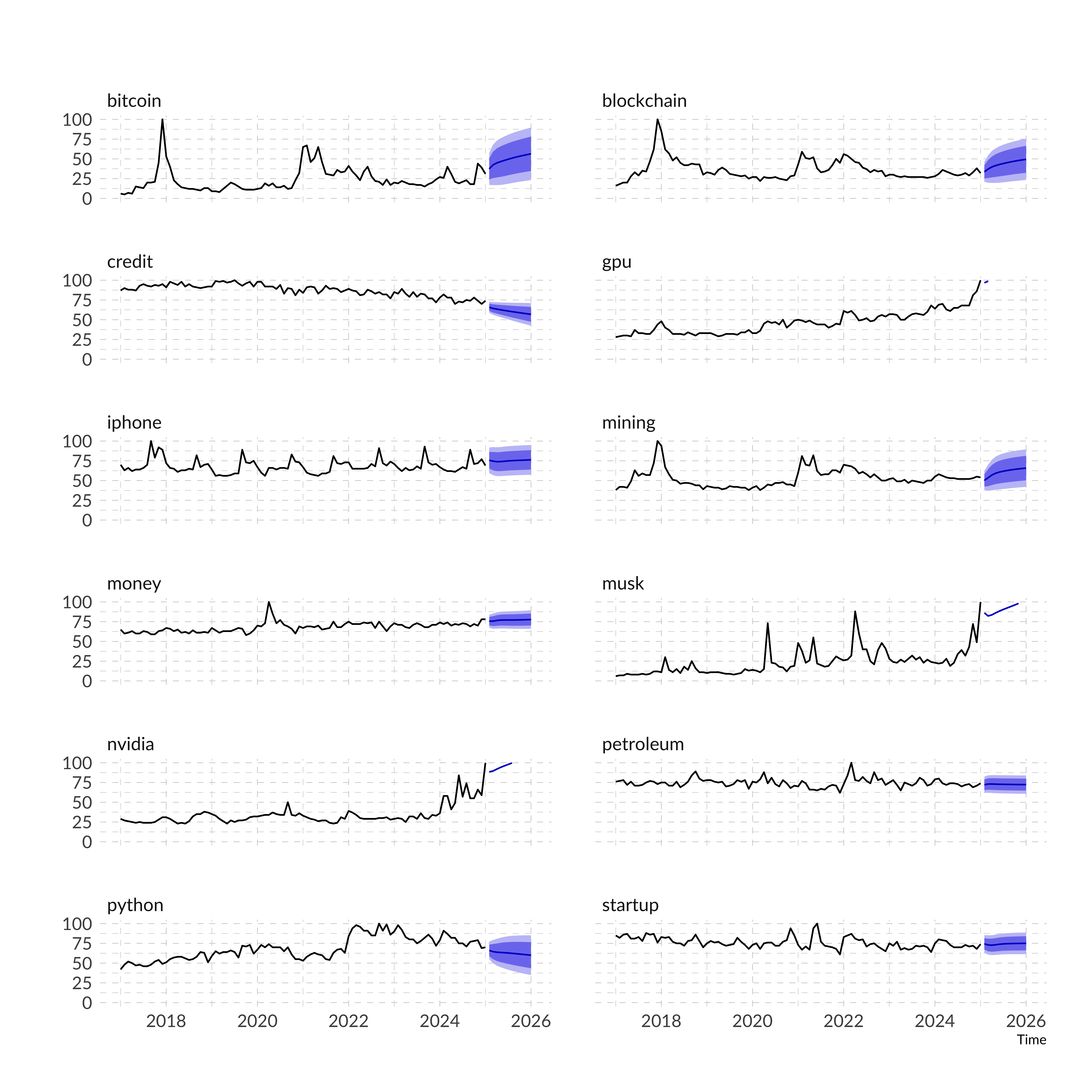
So, now we can create initial VAR-model with default parameters using all variables. VAR-models is provided in R by vars package. VAR function has a lot of parameters, but from my experience I can say that in most cases default parameters give the best result. The main parameter is the size of the lag - p. I have not yet had one case where its increase did not impair the result, therefore I keep it the default value.
It doesn’t look interesting, because all predicted trends are linear. To fix it I suggest taking the following steps:
add cross-validation for quality check;
add seasonality in model;
determine best variables for bitcoin trend prediction through cross-validation (we understand that often variables can be detrimental rather than helpful in forecasting).
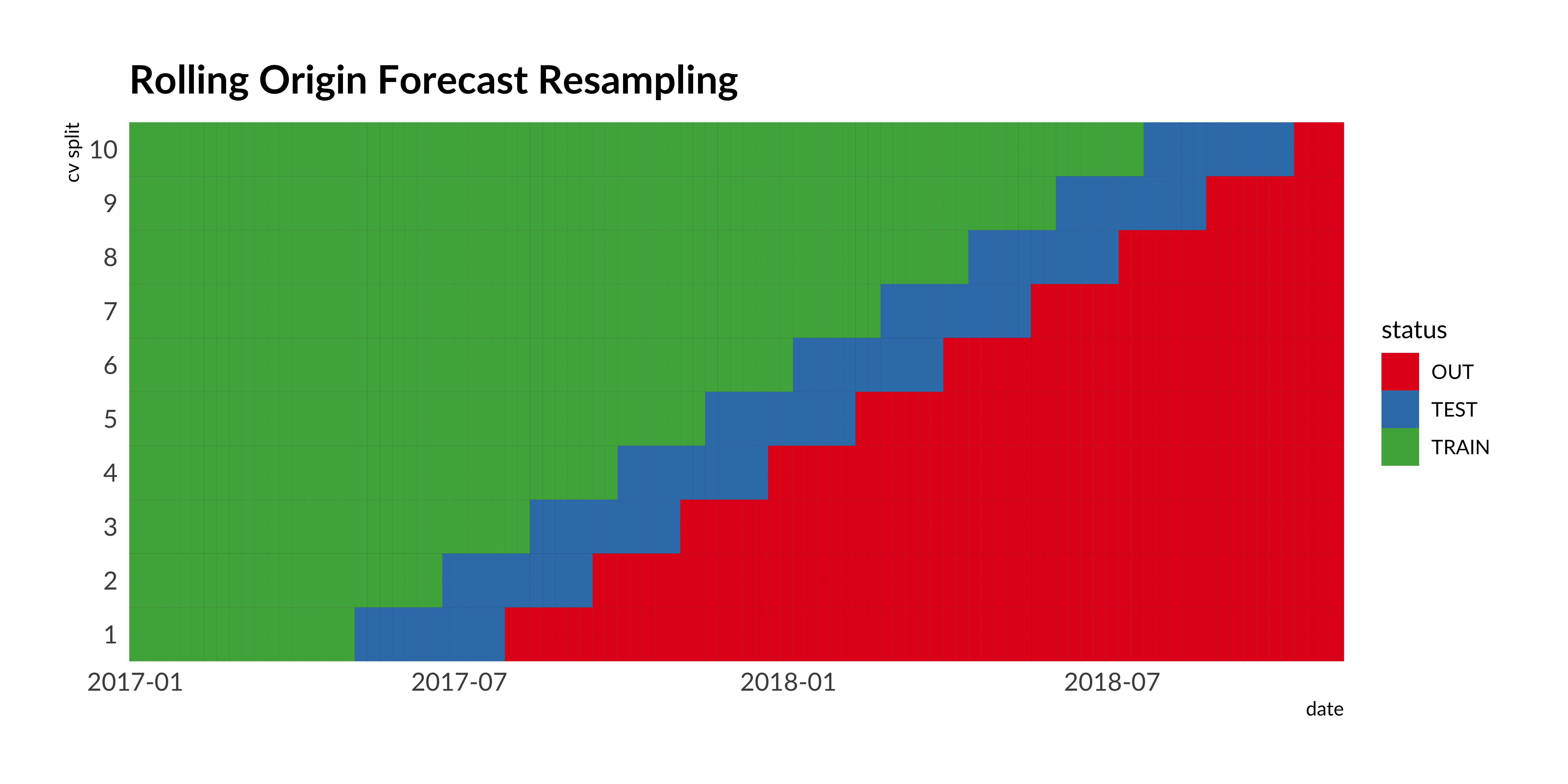
Let’s start with cross-validation. Time series models cross-validation doesn’t look like random or k-fold cross-validation for not time series data. We cannot shuffle all observations. We schould take the time order into account. In train split we can put only earlier dates than in test split. We will realise such logic using rolling origin cross-validation.
To split into train/test datasets we use rolling_origin function from rsample package.
Now we come to the main part of the post. Here I create function for cross-validation and variable selection in VAR.
I came up with a greedy approach to solving this problem. It has a few steps:
initialization of best_score (RMSE) and current iteration score;
initialization of goog variables list;
first iteration during which we select one variable with which the algorithm produces the best result, then we update best_score and best_current;
second (and more) iteration during which we select one more variable with which the algorithm produces the best result, the if new current score is better we update best_score, otherwise we quit.
Such approach allows you to determine the best combination of variables that best explain the dependent feature.
The best and in my case current method is cross-validation RMSE score. I understand that for forecasting it is more important to us that the model gives the best result on the freshest split. To take this into account I weigh the results on the split and give more weight to the split with the most up-to-date data. I do it using softmax function. For example, when I have 5 splits, last split has weight 0.64 and first split only 0.01.
To select good features using my greedy approach I create and run the next function:
Code
cv_search <-function(depend_variable, train_data, season = season_duration) { independ_variables <-colnames(train_data[[1]])[colnames(train_data[[1]]) != depend_variable] good_independ <-NULL best_score <-1000 best_current <-1000while (best_score == best_current) { g <- purrr::map_dbl(independ_variables, function(x) { k <- train_data %>% purrr::map(~vars::VAR(ts(.[, c(depend_variable, x, good_independ)]), p =1, season = season )) g <- purrr::map2_dbl( purrr::map(k, ~round(forecast::forecast(., window)$forecast$bitcoin$mean)), test %>% purrr::map(~.[[depend_variable]]),~Metrics::rmse(.x, .y) ) g %>%weighted.mean(w =softmax(c(1:length(g)))) }) result <-tibble(variable = independ_variables, mape = g) best_current <-min(result$mape, na.rm = T)if(best_score > best_current) { best_score <- best_currentcat(paste0("New best score = ", round(best_score, 3), "\n")) good_independ <-c(good_independ, result$variable[which.min(result$mape)])cat(paste0("Added new feature - ", result$variable[which.min(result$mape)], "\n")) independ_variables <- independ_variables[!(independ_variables %in% good_independ)] } }c(depend_variable, good_independ)}good_features <-cv_search("bitcoin", train)
New best score = 7.54
Added new feature - nvidia
This function returns an array of variables, which can best explain the dependent feature through vector autoregression. VAR-model with such variables gives 13.545 RMSE-score.
Let’s take a look at time series with these variables:
Code
time_series[, good_features] %>%head()
         bitcoin nvidia
Jan 2017       7     28
Feb 2017       6     27
Mar 2017       7     26
Apr 2017       6     25
May 2017      15     23
Jun 2017      16     25
So, our VAR eqution will look like \(bitcoin_t = bitcoin_{t-1} + startup_{t-1} + nvidia_{t-1} + musk_{t-1} + money_{t-1} + iphone_{t-1} + const + trend + seasonality\)
Although we have used other variables, the strongest and most statistically significant influence on the bitcoin trend still has the bitcoin trend itself.
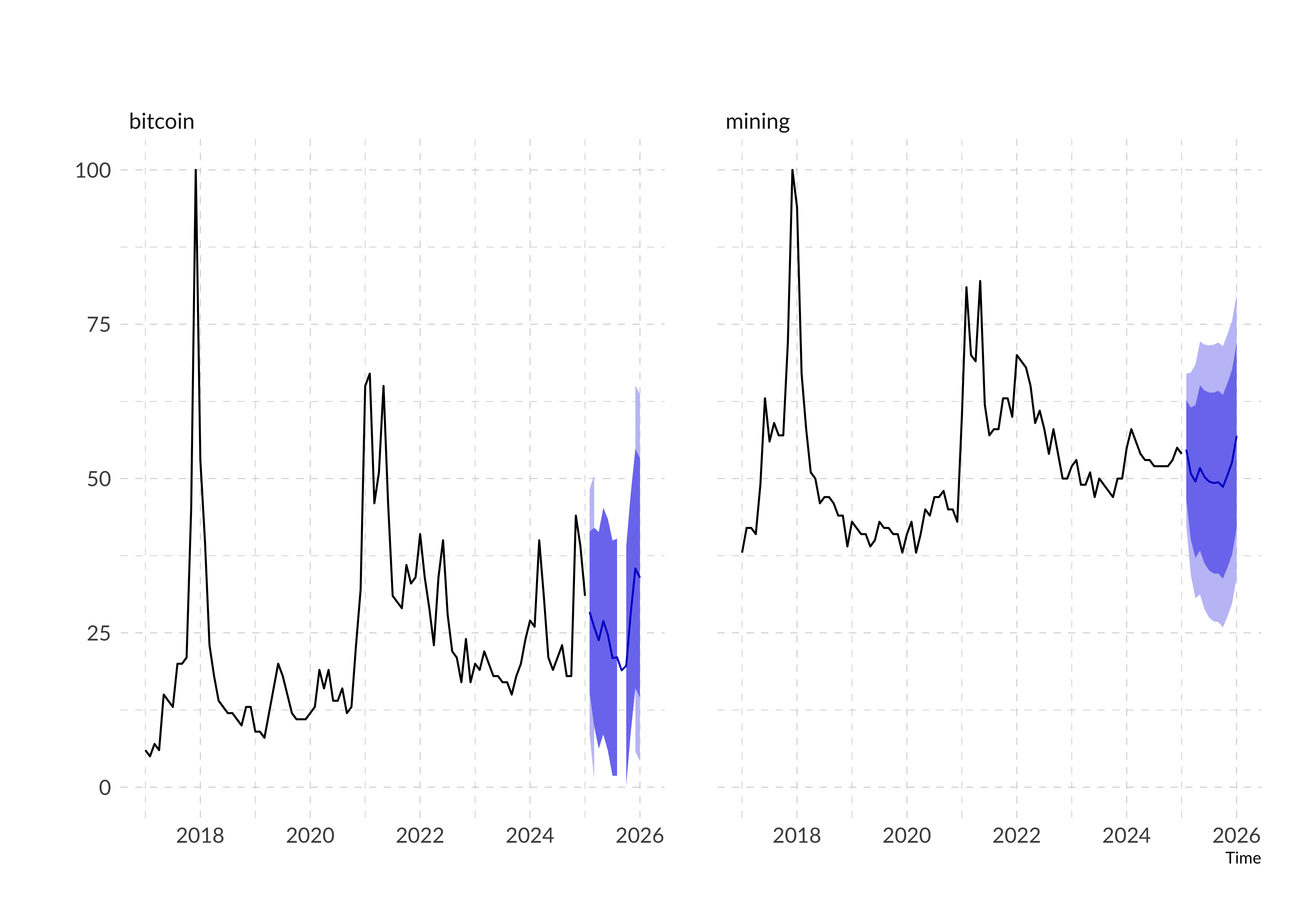
Now we can visualize the forecast for best features:
Compared to the first model it looks more attractive. Our model not only predicts the overall trend but also takes fluctuations in the year into account. But our main result is that we took the effects of other variables for the forecast into account, which is not provided by traditional time series forecasting methods. However, there is still a potentially better method for predicting multidimensional series - neural networks. However, it is better to apply them to large datasets, which we will definitely try to do in future.
Citation
BibTeX citation:
@online{kyrychenko2019,
  author = {Kyrychenko, Roman},
  title = {Time Series Prediction Using {VAR} in {R}},
  date = {2019-08-14},
  url = {https://randomforest.run/posts/var-time-series-analysis-using-r/var-time-series-analysis-using-r.html},
  langid = {en}
}
---title: "Time series prediction using VAR in R"description: | In this article I describe the main approach to create multivariate time series models. While univariate time series models are famous, they don't consider other factors.author: - name: Roman Kyrychenko url: https://www.linkedin.com/in/kirichenko17roman/date: 2019-08-14date-modified: 04-05-2023format: html: toc: true code-tools: truetwitter: creator: "@KyrychenkoRoman"categories: - time series - VAR - autoregression - visualizationscreative_commons: CC BYimage: "distill-preview.png"citation: true---```{r setup, include=FALSE}knitr::opts_chunk$set(echo = TRUE, message = FALSE, warning = FALSE)```**ARIMA, Exponential smoothing**.. are famous models for time series forecasting. But when you want to improve your model for ts-forecasting, it will be difficult for you to add new predictors in the model. It's a simple task for methods like linear regression, but not for time series forecast methods. Typical approaches for time series prediction include time series decomposition into trend, seasonality and noise, which are parts of a variable, that is interesting for us. It appears that we make time series prediction based on past values of the same feature. But current values depend not only on the same variable, but also on others variables.For example, we are interested in bitcoin trends. We can build a simple **ARIMA** model. To do this we need only bitcoin trends data. But bitcoin trends also depend on other trends like blockchain, mining, and nvidia as well. It makes real sense. Let's imagine that one week many people were searching for good nvidia GPU for bitcoin mining. THE next week the same people (who have good nvidia GPUs) were searching for minining, because they don't know how to do this. Then they will be looking for blockchain, because here they will mining bitcoins. So, googling for nvidia gpu causes googling for mining, and googling for mining gpu causes googling for blockchain. This is a theoretical model of behavior of users in Google. Such a model can be implemented using so called VAR-model. What is it?**VAR** is abbreviation for vector autoregression model. Roughly speaking VAR is an extended version of linear regression that contains lagged independ variables and variables for trend and seasonality description.$$y_t = c + A_1 y_{t-1} + A_2 y_{t-2} + \cdots + A_p y_{t-p} + e_t, \, $$Even the appearance of the formula is very reminiscent of multiple linear regression.So let's try to put this model into practice!Suppose you have multivariate time series like this:```{r setup and download data}suppressPackageStartupMessages({ require(dplyr) require(gt) require(ggplot2) require(hrbrthemes)})get_interest <- function(x){ gtrendsR::gtrends( x, time="2017-01-01 2025-01-01", onlyInterest = T)$interest_over_time %>% as_tibble()}bitcoin_trend <- purrr::map_dfr( c("bitcoin", "mining", "gpu", "money", "nvidia", "musk", "startup", "blockchain", "python", "petroleum", "credit", "iphone"), get_interest) %>% select(date, hits, keyword) %>% mutate(date = lubridate::date(date))head(bitcoin_trend) %>% gt() %>% tab_header( title = md("**Google trends**") ) %>% fmt_date( columns = c(date), date_style = 8 ) %>% tab_style( style = list( cell_fill(color = "white"), cell_text( align = "center", size = 3, font = "Lato")), locations = cells_body( columns = c("date", "hits", "keyword") )) %>% tab_style( style = list( cell_fill(color = "white"), cell_text( weight = "bold", size = 3, font = "Lato")), locations = cells_column_labels( columns = c("date", "hits", "keyword") )) ```This is data from Google trends collected with **trendyy** package.Lets convert this data to wide format:```{r explore}bitcoin_trend %>% tidyr::spread(keyword, hits) %>% head() %>% gt() %>% tab_header( title = md("**Google trends**") ) %>% fmt_date( columns = c(date), date_style = 8 ) %>% tab_style( style = list( cell_fill(color = "white"), cell_text( align = "center", size = 3, font = "Lato")), locations = cells_body( columns = c("date", "bitcoin", "mining", "gpu", "money", "nvidia", "musk", "startup", "blockchain", "python", "petroleum", "credit", "iphone") )) %>% tab_style( style = list( cell_fill(color = "white"), cell_text( weight = "bold", size = 3, font = "Lato")), locations = cells_column_labels( columns = c("date", "bitcoin", "mining", "gpu", "money", "nvidia", "musk", "startup", "blockchain", "python", "petroleum", "credit", "iphone") ))```So, we have 12 time serieses that is collected from Google trends. Notice data is weekly, therefore we set **season_duration** value to 52 (count of weeks in year). Also we cant to predict values for one year, so we set also forecast **window** to 52 (the equivalent of one year on our data set):```{r setup window}window <- 12season_duration <- 12```For best and fast data processing we need to convert this data from data frame to multivariate time series format. We can do it as follows:```{r ts object}time_series <- tsibble::as_tsibble( bitcoin_trend, index = date, key = keyword, regular = F ) %>% as.ts(frequency=12)```So, now we can create initial VAR-model with default parameters using all variables. VAR-models is provided in R by **vars** package. **VAR** function has a lot of parameters, but from my experience I can say that in most cases default parameters give the best result. The main parameter is the size of the lag - **p**. I have not yet had one case where its increase did not impair the result, therefore I keep it the default value.```{r initial var}var_model <- vars::VAR(time_series) summary(var_model)$varresult$iphone %>% broom::tidy() %>% mutate_if(is.numeric, round, 3) %>% gt() %>% tab_header( title = md("**VAR summary (bitcoin)**") ) %>% tab_style( style = list( cell_fill(color = "white"),cell_text(align = "center", size = 10, font = "Lato")), locations = cells_body( columns = c("term", "estimate", "std.error", "statistic", "p.value") )) %>% tab_style( style = list( cell_fill(color = "white"), cell_text(weight = "bold", size = 10, font = "Lato")), locations = cells_column_labels( columns = c("term", "estimate", "std.error", "statistic", "p.value") )) %>% data_color( columns = c(p.value), fn = scales::col_numeric( palette = c("#1a9850", "#d73027"), domain = c(0, 1) ) )```The output we get reminds the one of linear regression. Let's visualize the prediction:```{r trends, fig.width=10, fig.height=10, dpi=300}var_model %>% forecast::forecast(window) %>% forecast::autoplot() + scale_y_continuous(limits = c(0, 100)) + theme_ipsum(base_family = "Lato") + theme( panel.grid = element_line(linetype = "dashed") ) + facet_wrap(~series, scales = "fixed", ncol = 2)```It doesn't look interesting, because all predicted trends are linear. To fix it I suggest taking the following steps:- add cross-validation for quality check;- add seasonality in model;- determine best variables for bitcoin trend prediction through cross-validation (we understand that often variables can be detrimental rather than helpful in forecasting).Let's start with cross-validation. Time series models cross-validation doesn't look like random or k-fold cross-validation for not time series data. We cannot shuffle all observations. We schould take the time order into account. In train split we can put only earlier dates than in test split. We will realise such logic using rolling origin cross-validation.To split into train/test datasets we use **rolling_origin** function from **rsample** package.It has four arguments:- **data** - time series that may be split;- **assess** - size of the test split;- **initial** - minimal size of the train split;- **skip** - difference in size of the train splits.```{r rolling}rolling_cv <- rsample::rolling_origin( time_series %>% as_tibble(), assess = window, initial = window+round(window/2), skip = round(window/2) )rolling_cv```This function creates data frame with samples. For a better understanding I visualize it as follows:```{r rolling vis, fig.width=10, dpi=300}purrr::map_dfr( 1:nrow(rolling_cv), function(x) { tibble( split = x, id = c(rolling_cv$splits[[x]]$in_id, rolling_cv$splits[[x]]$out_id, (1:nrow(time_series))[!(1:nrow(time_series) %in% c(rolling_cv$splits[[x]]$in_id, rolling_cv$splits[[x]]$out_id))]), status = c( rep("TRAIN", length(rolling_cv$splits[[x]]$in_id)), rep("TEST", length(rolling_cv$splits[[x]]$out_id)), rep("OUT", length((1:nrow(time_series))[!(1:nrow(time_series) %in% c(rolling_cv$splits[[x]]$in_id, rolling_cv$splits[[x]]$out_id))])) ) ) }) %>% mutate( id = lubridate::as_date(id*7 + 17160)) %>% ggplot(aes(id, split, fill = status)) + geom_tile(color = "black", linewidth = 0.01) + scale_fill_manual(values = c("#e41a1c", "#377eb8", "#4daf4a")) + scale_y_continuous( limits = c(0.5, nrow(rolling_cv) + 0.5), expand = c(0,0,0,0), labels = c(1:nrow(rolling_cv)), breaks = c(1:nrow(rolling_cv)) ) + scale_x_date(expand = c(0,0,0,0)) + labs(title = "Rolling Origin Forecast Resampling") + ylab("cv split") + xlab("date") + theme_ipsum(base_family = "Lato")```We can see thath each train split is different by size.Let's create lists of train-test split data frames using rolling origin.```{r train_test}train <- rolling_cv$splits %>% purrr::map(rsample::analysis)test <- rolling_cv$splits %>% purrr::map(~rsample::assessment(.)[, 1])```Now we come to the main part of the post. Here I create function for cross-validation and variable selection in VAR.I came up with a greedy approach to solving this problem. It has a few steps:- initialization of best_score (RMSE) and current iteration score;- initialization of goog variables list;- first iteration during which we select one variable with which the algorithm produces the best result, then we update best_score and best_current;- second (and more) iteration during which we select one more variable with which the algorithm produces the best result, the if new current score is better we update best_score, otherwise we quit.Such approach allows you to determine the best combination of variables that best explain the dependent feature.The best and in my case current method is cross-validation RMSE score. I understand that for forecasting it is more important to us that the model gives the best result on the freshest split. To take this into account I weigh the results on the split and give more weight to the split with the most up-to-date data. I do it using softmax function. For example, when I have 5 splits, last split has weight 0.64 and first split only 0.01.You can check it from below:```{r}softmax <-function(z) exp(z) /sum(exp(z))softmax(1:5)```To select good features using my greedy approach I create and run the next function:```{r cv_search}cv_search <- function(depend_variable, train_data, season = season_duration) { independ_variables <- colnames(train_data[[1]])[colnames(train_data[[1]]) != depend_variable] good_independ <- NULL best_score <- 1000 best_current <- 1000 while (best_score == best_current) { g <- purrr::map_dbl(independ_variables, function(x) { k <- train_data %>% purrr::map(~vars::VAR(ts(.[, c(depend_variable, x, good_independ)]), p = 1, season = season )) g <- purrr::map2_dbl( purrr::map(k, ~round(forecast::forecast(., window)$forecast$bitcoin$mean)), test %>% purrr::map(~.[[depend_variable]]), ~Metrics::rmse(.x, .y) ) g %>% weighted.mean(w = softmax(c(1:length(g)))) }) result <- tibble(variable = independ_variables, mape = g) best_current <- min(result$mape, na.rm = T) if(best_score > best_current) { best_score <- best_current cat(paste0("New best score = ", round(best_score, 3), "\n")) good_independ <- c(good_independ, result$variable[which.min(result$mape)]) cat(paste0("Added new feature - ", result$variable[which.min(result$mape)], "\n")) independ_variables <- independ_variables[!(independ_variables %in% good_independ)] } } c(depend_variable, good_independ)}good_features <- cv_search("bitcoin", train)```This function returns an array of variables, which can best explain the dependent feature through vector autoregression. VAR-model with such variables gives 13.545 RMSE-score.Let's take a look at time series with these variables:```{r new ts}time_series[, good_features] %>% head()```So, our VAR eqution will look like $bitcoin_t = bitcoin_{t-1} + startup_{t-1} + nvidia_{t-1} + musk_{t-1} + money_{t-1} + iphone_{t-1} + const + trend + seasonality$Lets create model with only best features:```{r better var}better_var_model <- vars::VAR( time_series[, good_features], p = 1, type = "both", season = season_duration, ic = "FPE") summary(better_var_model)$varresult$bitcoin %>% broom::tidy() %>% mutate_if(is.numeric, round, 3) %>% gt() %>% tab_header( title = md("**VAR summary (bitcoin)**") ) %>% tab_style( style = list( cell_fill(color = "white"), cell_text(align = "center", size = 10, font = "Lato")), locations = cells_body( columns = c("term", "estimate", "std.error", "statistic", "p.value") )) %>% tab_style( style = list( cell_fill(color = "white"), cell_text(weight = "bold", size = 10, font = "Lato")), locations = cells_column_labels( columns = c("term", "estimate", "std.error", "statistic", "p.value") )) %>% data_color( columns = c(p.value), colors = scales::col_numeric( palette = c("#1a9850", "#d73027"), domain = c(0, 1) ) )```Although we have used other variables, the strongest and most statistically significant influence on the bitcoin trend still has the bitcoin trend itself.Now we can visualize the forecast for best features:```{r vis effects, fig.height=7, fig.width=10, dpi=300}better_var_model %>% forecast::forecast(window) %>% forecast::autoplot() + scale_y_continuous(limits = c(0, 100)) + theme_ipsum(base_family = "Lato") + theme( panel.grid = element_line(linetype = "dashed") ) + facet_wrap(~series, scales = "fixed", ncol = 2)```Compared to the first model it looks more attractive. Our model not only predicts the overall trend but also takes fluctuations in the year into account. But our main result is that we took the effects of other variables for the forecast into account, which is not provided by traditional time series forecasting methods. However, there is still a potentially better method for predicting multidimensional series - neural networks. However, it is better to apply them to large datasets, which we will definitely try to do in future.